1. Introduction
The idea here is to apply the idea of “gossip”, that is locally distributed messages, to facilitate an evolutionary algorithm. In this approach it is the whole population of ‘solutions’ that learns how to solve a problem – the population is not just a vehicle for evolving the ‘best’ global solution. Thus, although the proposed approach can be interpreted as the adaptive propogation of solutions (or “memes”) within a population spread across different local conditions, it has an application as a truly distributed evolutionary learning algorithm.
2. The Idea and the Technique
The idea of this technique is that there is a space in which the potential solutions or memes are distributed. Each “location” or “region” of the space is associated with a different part of a problem domain. At each location in the space there is a local competition and evolution of these memes or solutions. Thus the algorithm attempts to learn what solutions work best for each part of the problem in parallel. Solutions that are locally successful propogate to neighbouring (overlapping) locations where it has to compete with the other solutions there. If there is an accessible global solution it will eventually propogate to all locations, whilst solutions which have a more limited scope will only successfully propogate to those problem areas where they work relatively well. At the end of the process, it may well be that there is no single solution that globally dominates, but different solutions may be found to work better in different parts of the problem domain. If a global solution is required then this can be constructed by analysing the whole population that develops. That is, by finding the best solution at each location and forming a composite solution from these using conditions of application for each.
This is analogous to how human societies have developed different ways of exploiting the environment in the different geographical niches in which it has spread (Reader 1990). This variety of methods does not stop regions learning from their neighbours where this is useful. Thus some techniques (such as the use of fire) have spread to all parts of the globe, whilst others (such as hunting with harpoons) are only found in particular areas.
The technique, at its most basic, consists of two phases: a development stage followed by an analysis phase. In the development phase there must be a population of solutions spread across different locations forming a series of small overlapping localities, such that each locality can be associated with a different sub-problem (or subdomain of a problem). Repeatedly, in each locality, the solutions are evaluated on the associated sub-problem or sub-domain and solutions selected and replicated in that locality. The localities must overlap so that solutions that are successful in one locality can spread through neighbouring localities, and potentially the whole space.
The analysis phase takes the resulting population of solutions and analyses it in order to extract useful information. This might involve identifying the best solution in each locality and combining them together to form a complex composite solution.
This technique, as with all techniques, has advantages, and disadvantages – this can be seen as a consequence of the “No Free Lunch” theorems (Wolpert and Macready 1997, Culberson 1998). On the plus side it: uses to the maximum extent the information about the problem that is encoded in the whole population of solutions and not just that in the single best solution; the technique is only evaluated locally which is compuationally efficient; complex compond (total) solutions can be evolved with relatively small genes, and it is eminently suitable for massively parallel execution (each locality could be on a separate processor with no need for global communication). Disadvantages include the need for an analysis stage after the development phase has finished, and the fact that the way the problem space is decomposed into localities can effect the effectiveness of the approach.
Let me illustrate the approach with a simple curve fitting example. Imagine that one has a set of points and one is trying to evolve the curve that fits these points the best. In a global approach (Figure 1), the solutions attempt to fit all the points simultaneously and hence are evalutated across the whole domain of points each time.
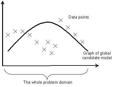
Figure 1. Graph fitting example – trying to fit some points with a single curve
In the distributed learning approach propounded in this paper, the domain is divided up into a number of different (overlapping) neighbourhoods and the solutions evolved and evaluated only at those localities. This is illustrated in Figure 2. If one wanted a global solution one would have to construct it “piecemeal” from the best fitting curves in each locality – one could see this as a sort of Genetic Programming version of local regression (Cleveland and Devlin 1988).
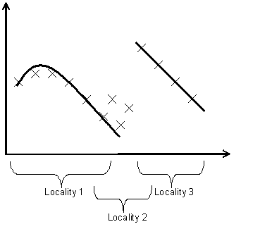
Figure 2. Graph fitting example - fitting the points with two different solutions in two localities
3. Model Setup
In this case the problem was predicting the outcomes of heart disease in a set of data from Patients in Cleveland. There were four possible outcomes: 0, 1, 2, 3, 4 to be predicted on the basis of 13 other attributes, all numeric or coded as numbers.
The approach was based on Genetic Programming (Koza 1992, 1994). Each gene was composed of 5 numeric expressions (one for each possible outcomes), coded as trees. Possible functions in these trees include basic arithmetic and comparison operations. The leaves include a selection of constants and the values of the 13 attributes. Evaluation is done given a set of values for the 13 “predictive” attributes by evaluating the 5 functions – the greatest value indicating which outcome is indicated. When two genes are crossed, there is a probability that each corresponding tree will be crossed.
Thus the nodes (i.e. the functions) in the trees were as follows: IGZ (if arg1 >0 then arg2 else arg3), MAX (the maximum of two values), MIN, MINUS, PLUS, SAFEDIVIDE (arg1/arg2 unless arg2=0 then is 0), TIMES. The leaves of the trees were either a variable (INPUT 1, INPUT 2, …, INPUT 13) or a constant (-1, -0.9, -0.8, …, -0.1, 0, 0.1, …, 0.9, 1).
Constant parameters across all types of run were:
· Initial tree depth = 3
· Number of neighbours = 4
· Predictor feature positions = [1 2 3 4 5 6 7 8 9 10 12 13]
· Predicted feature position = [14]
· Number of independent runs = 12
The algorithm presented is called the local algorithm, in contrast to a corresponding GP algorithm which is the global version. The local algorithm is divided up into a development (i.e. exploratory) phase and an analysis (i.e. exploitative) phase. These are outlined below.
The local algorithm setup
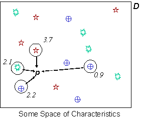
The working of this algorithm is illustrated in
Figure 3. If you imagine that every point is a person who may be invaded by a meme which are distributed close by, the one that is best for that person (in their situation) is selected (or mixed from the best). This repeatedly happens allowing the gradual spread of solutions across the space by (mostly) local propagations and crossings.
Figure 3. An Illustration of the working of the development phase. The problem space (D) is scattered with different solutions (the different shapes); each instant: a random point in the space (D) is chosed (p); some solutions nearby (and at the point) are selected (circled); they are evaluated at p giving the fitnesses (numbers by each circle); the fittest are selected (bold circles) and crossed (or propagated); the result placed at the point.
An outline for the algorithm is as follows:
Initialise space with a random set of genes
Repeat
For geneNum from 1 to popSize
Randomly select a locality
randomly select from locality
a set of sample genes
evaluate set in the locality
chose two best from set
if randomNum < probCrossover
then cross two best -> newInd
else best -> newInd
Next geneNum
New population composed of newInds
Until finished
For efficiency a neighbourhood relation was imposed upon the space of possible positions in the context space, by giving each possible position in the space a set of 4 of the nearest neighbours (judged by a hamming distance). In early experimentation on the topology I found that the exact distance metric did not noticeable effect the results. This pre-compiled neighbourhood relation eliminated the overhead of recalculating who were the closest neighbours of any point. In this version of the algorithm, the random selection of solutions in the locality (mentioned in the algorithm outline above) are: a random selection of solutions at the neighbouring localites plus all those at the chosen locality.
Parameter settings for the development stage of local runs were:
· Density (number at each locality) = 5
· Number of Generations = 30
· Number of sample in locality not at chosen location = 3
· Crossover probability = 0.2
Parameter settings for the analysis stage of local runs were:
· Density (number at each locality) = 1
· Number of Generations = 170
· Number of sample in locality not at chosen location = 5
· Crossover probability = 0
Thus in the analysis stage solutions are only propagated to those localities where they are best, no new solutions are generated. The number of generations for this stage was probably excessive, as we will see later (Figure 5 and Figure 6).
The global algorithm setup
This was a straight GP algorithm using the same gene structure as above. Each generation each algorithm was only evaluated against 10% of the total data set, since that made the GP algorithm more competative against the local algorithm. Election was used so the best solution at any point was carried over to the next generation. Other parameters were:
· Population = 280
· Number of Generations = 20
· Number of sample in locality not at chosen location = 3
· Crossover probability = 0.9
The smaller population and number of generations was chosen so that the number of evaluations would be comparable to those in the local runs. I did try it with larger populations and for longer but the results were not better in terms of effective error against number of evaluations.
4. The Data Set/Test Problem
The Data Set that the technique was tested upon was that concerning heart disease in Cleveland, US available at the ML repository of problems. This was chosen a random from those available. The data I used consisted of 281 examples of 14 numeric attributes, including the predicted value coded: 0, 1, 2, 3 or 4 depending on the actual outcome. The problem is to predict the outcome given the other 13 values of the characteristics. Attributes refered to in the paper are 1, 2, 4 and 5 which stand for the age, sex, resting blood pressure in mm Hg on admission to the hospital (trestbps), and serum cholestoral in mg/dl respectively (chol). Thus the spaces I tried for the space of solutions were {age, sex} and {trestbps, chol} – these selections were pretty arbitrary, simply based on a quick inspection of the values and not based in any way upon knowledge of what the important factors are. More details about the data set can be found in appendix 1.
5. Results
Three sets of runs were done. The first was a standard GP algorithm “Global” (12 runs); the second using the local algorithm above with the context space being defined by attributes 1 and 2 “Local (1, 2)” (12 runs); the second using the local algorithm above with the context space being defined by attributes 4 and 5 “Local (4, 5)” (12 runs).
Comparing the different algorithms is not entirely straightforward. The purpose of the GP algorithm (Global), is to evolve the best global solution. Thus its effective error is the error of the best solution measured by that solution’s average error over the whole problem. The pupose of the algorithm proposed here is to evolve local solutions. Thus its effective error is its average error of the best local solutions in each locality when evaluated over their local spaces. Also the local algorithm involves orders of magnitude less computational time per generation for the same population size, so comparing the effective error rate per generation would be misleading. The overwhelming overhead in this (and all) evolutionary algorithms is the time taken to evaluate each solution. It is this comparison which is shown in Figure 4. To give the Global runs more of a chance each time a solution is evaluated it does so against a random sample of only 10% of the total population (though in the statistics below the error is a truly global evaluation). With respect to the effective error against the number of evaluations the performance of the Global approach was even worse when each (new) solution was evaluated against the whole problem rather than just a sample, since although the effective error achieved was slightly better, the number of evaluations this took was roughly 10 times greater. Thus I calculate each run’s effective error against the number of evaluations it takes. The dense, flat regions at the end of the Local sets is the analysis stage where the generality of discovered solutions occurs. This is included in the graph below because this stage is a necessary overhead in the local approach proposed.
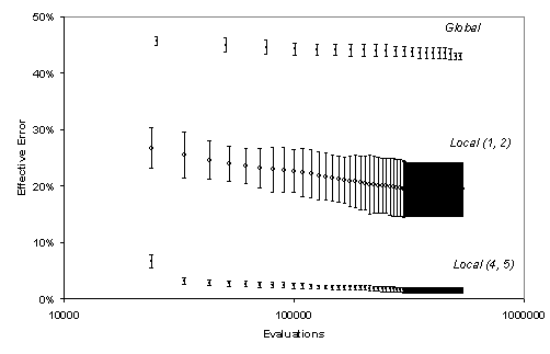
Figure 4. A comparison of effective error rates in the three sets of runs against the number of evaluations it takes (circles are averages, with the error bars indicating one standard deviation adjusted for sample size)
As you can see in Figure 4, The two Local runs significantly out-perform the Global runs. That is, for the same computational expense the average local errors of the current locally best solutions in the Local runs are significantly less than the average global error of the single best current solution in the Global runs. But what is also interesting in these results is the difference that the chosen problem space has on the effectiveness of the algorithm. The Local algorithm did much better when done using the space defined by attributes 4 and 5 than when using the space defined by attributes 1 and 2.
Figure 5 and Figure 6 show the average effective error and the average spread of the Local (1, 2) and Local (4, 5) runs respectively. Here the spread is the number of localities that a solution occupies in the space. Thus an average spread of 2 would mean that there were twice as many solutions in the space as unique solutions. In these figures the development and analysis phases are clearly shown. In the development phase there is a low average spread as new (unique) solutions are continually being generated, but the appearance of new solutions makes the gradual decrease in error possible. In the analysis phase there are no new solutions being generated but only local propogation of solutions, so that they ‘fill out’ the areas of the space that they perform best in, so the effective error rate is flat. In this phase the spread increases as the best solutions occupy the surrounding locations where they also dominate.
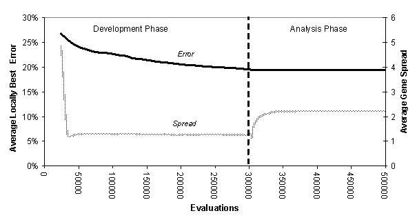
Figure 5. The average (over 12 runs) of the effective error rate and gene spread for Local (1, 2)
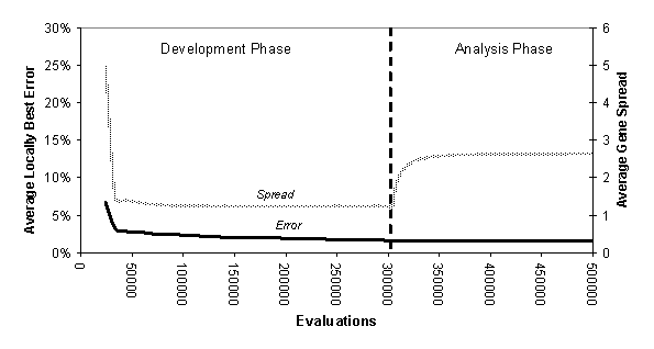
Figure 6. The average (over 12 runs) of the
effective error rate and gene spread for Local
(4, 5)
In Figure 5 and Figure 6 one can see that not only did the Local(4, 5) runs have a far lower effective error than the Local(1, 2) runs but also that they ended up with a slightly higher average spread. That means that the Local(4, 5) runs achieved (on average) a greater level of generality than the Local(1, 2) – there was no trade-off between error and generality between these two, the later was better in both respects.
Figure 7 and Figure 8 are illustrations of the sort of local spread of solutions that have occurred by the end of the analysis phase. In these only the more numerous solutions are shown so that their ‘domains’ are easily distinguishable.

Figure 7.
The attribute distribution of the more numerous best genes (those
occuring more than once) in the run with the smallest effective error for Local (1, 2)
Figure 7 shows the positions in the problem space determined by the attributes 1n and 2, that is of age (horizontal axis) and sex (vertical axis – only male top, both middle, only female bottom) of all the best solutions (in the run with the best effective error) that occurred more than once. One can see some significant clustering by age but not so much by sex.
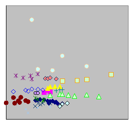
Figure 8. The attribute distrinbution of the more
numerous best genes (those with at least 4 occurences) in the run with the
smallest effective error for Local (4, 5)
Figure 8 shows the positions in the problem space determined by the attributes 4 and 5, that is of resting blood pressure (trestbps - horizontal axis) and serum cholestoral (chol - vertical axis) of all the best solutions (in the run with the best effective error of 1.07%) that occurred more than thrice. Here we see pronounced clustering by in both dimensions, but perhaps more by chol than trestbps.
The fact that in Local (4, 5): both dimensions facilitated pronounced clustering; there was a greater total number of localities; and there was greater connectivity were probably factors its success compared with Local(1, 2.
6. Discussion
Although Local (1, 2) did better in terms of effective error than the other runs and better than some previous ML attempts (see Appendix 1), this is not an entirely fair comparison because they are aiming at different sorts of outcome, i.e. global solutions of a certain type. Clearly by simply approximating the oringinal table of data one would obtain a zero level of error using an entry-by-entry level of locality. However, as one can see from Figure 7 and Figure 8, at least some level of generality above an entry-by-entry level has been achieved. There is presumably (for each problem) some sort of three-way trade-off between: the generality of the solution one obtains; the efficiency of the distributed search; and the level of effective error. Presumably by adjusting the parameters in the local approach one can obtain different levels of generality and explore this trade-off (something I have not done). This might be exploited by a gradual increase in the level of locality as the process progresses – rather like the “cooling” regime in simulated annealing.
Given the strength of the analogies with ecological systems and the efficiency of the approach, one wonders why this approach has not been thought of before. Perhaps this is due to a bias towards the search for the most general solution possible regardless of its cost in terms of other desirable attributes.
7. Related Work
The algorithm was originally published as (Edmonds 2001) but applied and interpreted in a different way to that here. There it was developed as a step towards solving the problem of learning appropriate cognitive contexts arising from the analysis of the roots of context in (Edmonds 1999).
The model has a close relation to that of “demes” in evolutionary programming (Tanese 1987). There the space of solutions is split into a series of islands (where the evolution occurs), there being allowed only a slow rate of migration between islands. This technique acts to preserve a greater level of variety in the total population of solutions than would be the case if they were all evolved together. However in that technique the solutions in each island are evaluated globally against the whole problem space. It is particularly closely related to the diffusable cooperative coevolutionary genetic algorithms (DCCGA) of (Wiegand 1999). In CCGA (Potter and de Jong 1994, Potter 1997) the population is divided up into subpopulations, each of which is evolved to solve a designated sub-problem of the whole. Spears (1994), identified the separate sub-populations using “tags” allowing some drift between sub-populations using a low rate of mutation in these tags. Wiegand (1999) combines these techniques so that some diffusion between populations is added to CCGA resulting in DCCGA. However, in DCCGA: the separate solutions in each population are still evaluated with respect to the whole problem (along with other solutions to other sub-problems); the sub-populations are determined in advance by the programmer; and there is no space to structure the diffusion of solutions with respect to the relation between sub-problems.
It also is related to clustering algorithms, in that it divides up the domain into those where particular solutions can dominate (e.g. Kaufmann and Rousseeuw 1990). However unlike these which cluster based on some assumptions about the characteristics of data, this approach co-evolves the solutions with the clusters, allowing the discovery of clusters with respect to unexpected relations to be identified.
This model has an obvious and close ecological interpretation – e.g. those in (Wright 1932, Vose and Liepins 1991). The localities can be seen as the various niches (localities in the problem space) which the different species (the different solutions) compete to occupy. Successful species will tend to spread out over the areas in which they are competative. After a while mutuation will cause speciation amoung the most populous species in any set of localities and these new, closely related, species will then start to compete anew. This dunamic is described in (Edmonds 2001). Of course, just as with nature, areas which are particularly difficult to exist within may exist, in which there are no well-adapted species whilst other, easier, environments may have many fit species.
8. Conclusion
All search techniques exploit some trade-off or other. This technique trades in the generality of a single solution in return for a more efficient algorithm and information about the problem structure. Instead of a uniform, single solution one gets a composite solution by analysing the resulting whole population. Although the space within which problems will evolve can greatly effect the quality of the solution that resuls, one does not have to explicitly divide up this space into specific subproblems, but areas that are solvable using the same local solution coevolve with the content of the solutions.
Acknowledgements
Thanks to the participants of the Internation Conference on Modelling and Using Context, for valuable discussions on these and related ideas.
References
Aha, D. and Kibler, D. Instance-based prediction of heart-disease presence with the Cleveland database. Technical Report, University of California, Irvine, Department of Information and Computer Science, Number ICS-TR-88-07, p. 8, March 1988.
Blake, C.L. & Merz, C.J. (1998). UCI Repository of machine learning databases. Irvine, CA: University of California, Department of Information and Computer Science. www.ics.uci.edu/~mlearn/MLRepository.html
Cleveland, W. S. and Devlin, S. J. (1988) Locally-weighted regression: An approach to regression analysis by local fitting, J. Am. Statist. Assoc. 83 596 - 610.
Culberson, J. On the Futility of Blind Search: An Algorithmic View of 'No Free Lunch', Evolutionary Computation 6 (1998): 109–27.
Detrano, R. et al. Internation application of a new probability algorithm for the diagnosis of coronary artery disease. American Journal of Cardiology 64:304-310, 1989.
Edmonds, B. The Pragmatic Roots of Context. in Bouquet, P.et al. (eds.) Modeling and Using Contexts: Proceedings of the 2nd International and Interdisciplinary Conference, Springer-Verlag, Lecture Notes in Artificial Intelligence, 1688:119-134, 1999.
Edmonds, B. Learning Appropriate Contexts. in Akman, V. et al. (eds.) Modelling and Using Context: Proceedings of the 3rd International and Interdisciplinary Conference, Springer-Verlag, Lecture Notes in Artificial Intelligence, 2116:143-155, 2001.
Gennari, J. H. Langley, P. and Fisher, D. Models of incremental concept formation, Artificial Intelligence, 40:11-61.
Kaufman, L. and Rousseeuw, P. J. (1990) Finding roups in data: and introduction to cluster analysis, John-Wiley & Sons.
Koza, J. R. Genetic Programming: On the Programming of Computers by Means of Natural Selection. MIT Press, Cambridge, MA, USA, 1992.
Koza, J. R. Genetic Programming II: Automatic Discovery of Reusable Programs. MIT Press, Cambridge, MA, USA, 1994.
Potter, M. A. The Design and Analysis of a Computational Model of Cooperative Coevolution (Doctoral dissertation, George Mason University). (1997)
Potter, M. A. and De Jong, K. A Cooperative Coevolutionary Approach to Function Optimization. In: The 3rd Parallel Problem Solving from Nature (PPSN), Proceedings of the Conference. Springer-Verlag, New York (1994) 249-257
Reader, J. (1990) Man on Earth. Penguin Books.
Spears, W. “Simple subpopulation schemes”. In: Proceedings of the 3rd Conference on Evolutionary Programming. World Scientific (1994) 297-307.
Tanese, R. (1987) Parallel genetic algorithms for a hypercube. In Grefebstette, J. J. (ed.), Genetic Algorithms and their Applications: Proceedings of the 2nd International conference on genetic algorithms, Hillsdale, NJ: Lawrence Erlbaum, 177-183.
Vose, M. D. and Liepins (1991) Wright’s shifting balance theory: an experimental study. Science 253:1015-1018.
Wiegrad, R. (1999) Applying Diffusion to a Cooperative Coevolutionary Model. Parallel Problem Solving from Nature PPSN V 5th Internation Conference, Springer, LNAI ??
Wolpert, D. H. and Macready, W. G. No Free Lunch Theorems for Optimization, IEEE Transactions on Evolutionary Computation 1 (1997): 67–82.
Wright, S. (1932) The roles of mutation, inbreeding, crossbreeding and selection in evolution. In Proceedings of the 6th International Congress of Genetics, vl. 1, 356-366.
Appendix 2 – The Data Set
The information given below is culled from the information file that comes with the data set at the Repository of machine learning databases (Blake and Merz 1998). I include it for completeness – I have almost no knowledge of heart disease.
Title
Heart Disease Databases (processed Cleveland subset)
Source Information:
· Creator: V.A. Medical Center, Long Beach and Cleveland Clinic Foundation: Robert Detrano, M.D., Ph.D.
· Donor: David W. Aha (aha@ics.uci.edu) (714) 856-8779
· Date: July, 1988
· Obtainable from: www.ics.uci.edu/~mlearn/MLRepository.html
Past usage
(Detrano et al 1989) achieve approximately a 77% correct classification accuracy (i.e. 23% error) with a logistyic-regression-derived discriminant function on similar data sets. (Aha and Kibler) achieved a 77% accuracy with Ntgrowth and 74.8% accuracy with C4, using instance-base prediction of heart-disease presence. (Gennari, Langley and Fisher 1989) achieved a 79.9% accuracy using their CLASSIT conceputal clusering system.
Summary
This database contains 76 attributes, but all published experiments refer to using a subset of 14 of them. There are, in fact, four data sets from different parts of the world, but the Cleveland database is the only one that has been used by ML researchers to this date. The "goal" field refers to the presence of heart disease in the patient. It is integer valued from 0 (no presence) to 4. Experiments with the Cleveland database have concentrated on simply attempting to distinguish presence (values 1,2,3,4) from absence (value 0).
There are 303 instances, but this includes fields with missing data. The subset used here were the 281 with complete data. The total number of attributes was 76, but only 14 were used here.
Attributes
Only 14 used. The hashed number is the attribute number in the complete set.
1. #3 (age): age in years
2. #4 (sex): sex (1 = male; 0 = female)
3. #9 (cp): chest pain type
Value 1: typical angina
Value 2: atypical angina
Value 3: non-anginal pain
Value 4: asymptomatic
4. #10 (trestbps): resting blood pressure (in mm Hg on admission to the hospital)
5. #12 (chol): serum cholestoral in mg/dl
6. #16 (fbs): (fasting blood sugar > 120 mg/dl) (1 = true; 0 = false)
7. #19 (restecg): resting electrocardiographic results
Value 0: normal
Value 1: having ST-T wave abnormality (T wave inversions and/or ST elevation or depression of > 0.05 mV)
Value 2: showing probable or definite left ventricular hypertrophy by Estes' criteria
8. #32 (thalach): maximum heart rate achieved
9. #38 (exang): exercise induced angina (1 = yes; 0 = no)
10. #40 (oldpeak): ST depression induced by exercise relative to rest
11. #41 (slope): slope: the slope of the peak exercise ST segment
Value 1: upsloping
Value 2: flat
Value 3: downsloping
12. #44 (ca): number of major vessels (0-3) colored by flourosopy
13. #51 (thal): 3 = normal; 6 = fixed defect; 7 = reversable defect
14. #58 (num) (the predicted attribute): diagnosis
