Bruce Edmonds,
Centre for Policy Modelling
Manchester Metropolitan University,
All Saints Campus, Oxford Road, Manchester, M15 6BH, UK
Tel. +44 161 247 6479
Email: bruce@edmonds.name
Abstract
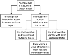
A complex individual-based meta-population simulation is presented which allows the exploration of systemic change within an ecosystem. This model exhibits a variety of different states but can show the build up of multi-trophic levels of food web and dynamics of species. The model is composed of a set of patches, each well mixed, with slow rates of migration occurring between neighbouring patches. The impact of humans upon this is done in two different ways: firstly by the systematic “blocking” of dimensions of inter-species interaction and, secondly, by the introduction of individuals to represent humans which have a social (rather than genetic) set of affordances. The outcomes of such experiments is analysed at a number of levels. The results show that although some general relationships between settings and outcomes are discernable, some of the meaningful patterns are context-specific. Some hypotheses about the conditions that maintain some ecological diversity despite the impact of human individuals are suggested.
Graphical Abstract
Highlights
· Risk-oriented analysis of a complex model of human-ecology interaction
· A combined individual-based model including plants, herbivores, predators as a base for the exploration of the complex impacts of humans
· Two different ways of introducing systemic change: (a) by changing (blocking) dimensions of the interaction structure and (b) by introducing individuals representing humans
· Analysis of impacts at a number of different levels including: example simulation states, trajectories, sensitivity analysis, data-mining of a large number of random runs, and specific explorations starting from the same initial ecological state
· Reveals context-dependency of some of the significant effects, suggesting that simpler models might have missed these
· Suggests a number of hypotheses for preserving ecological diversity under the impact of humans
Keywords
Individual-based
simulation, ecology, human impact, systematic change, risk analysis
Software availability
The simulation and its code will be available from http://cfpm.org/models/ems from the 18th June 2013. Once the code has been cleaned and ODD documentation for this is complete it will be posted to openabm.org under the title “A multi-patch meta-population of an ecology with humans”.
1. Introduction
Due to their abilities, groups of humans can inhabit a variety of ecological niches. They do this by adapting to a niche in terms of developing a body of knowledge, including words, ideas, techniques, social norms, systems of value and ways of organising, that enables the group to survive there01990). Once established this body of knowledge can be passed down to new members of the group so that the group can retain its ability to survive in that niche over time. Broadly this set of knowledge can be associated with the culture of the group. Thus the adaptivity of groups of humans can occur far more rapidly than that of most animals that have to rely on genetic evolution for their adaption. Humans are thus at a distinct advantage in terms of any adaptive “arms race” with other species. However, they do not necessarily plan for the long-term and can cause such a degree of environmental damage to the niches they inhabit that they endanger the survival of their own group (Diamond 2004). In this way the arrival of humans within a system of ecosystems can have a profound impact upon it. Thus, the arrival of humans is a prime example of systemic change within ecosystems – it does not merely change the extent of extinction but also the way the dynamics of that ecosystem work.
However, how this arrival will effect a particular ecosystem is not always clear – sometimes it seems that a balance between humans and the rest of the ecosystem is established, but at other times the arrival of humans can only be described as catastrophicError! Reference source not found.. This paper presents a couple of ways in which such systematic change can be explored within and individual-based meta-population model. The purpose of this is to start to detangle the various complex impacts. This is a kind of risk analysis, looking for possible ways in which such a system could fail[1]. It is not a probabilistic representation, but a possibilistic one – it suggests complex hypotheses concerning how the interactions within the complex of ecology+humans might occur. The model variants exhibited below show, once again, how the impact of such systemic change within complex systems is hard to predict and can be very context-specific. It also shows that it can be important to simulate ecological and human aspects all together rather than simulating an ecology with a simple fix “add on” to represent human impact (or vice versa). With complex systems putting together two models can produce patterns of outcomes that are not apparent in either model separately.
Clearly this model, although it does reproduce some observed phenomena in vague qualitative ways, is not a descriptive representative model. It does not describe reality in terms of what does happen, only in what sort of things might happen and why.
The main body of the paper is divided into three sections: section 2 describes the underlying ecological model, section 3 looks at the first approach to introducing systemic change by interfering with the underlying structure of interactions between species, and section 4 looks at the second approach where individuals representing humans are introduced within evolved ecologies. Each of these sections includes a description of the approach, the relevant results and a short discussion. This is followed by a more general discussion of these results (section 5) and the conclusions (section 6). This is followed by two appendices containing more details about the simulation, section 7, and some sets of results not included in the main text, section 8[2].
2. The Basic Meta-Population Ecological Model
First the basic model of the ecology is presented. This model is then altered/extended in a couple of ways to explore the impact of humans upon the outcomes in this model.
2.1 The Method
This is a synchronous individual-based simulation. In this, entities, plants, herbivores and predators, are represented as individual objects. They inhabit one of a number of patches arranged in a 2D pattern that makes up the world. Each patch is well mixed so that interactions within that patch are random, but there is a probability that each individual can migrate to one of the four neighbouring patches each tick. The world is wrapped vertically and horizontally. Each patch and individual has a binary bit-string that represents its characteristics, their lengths determined by parameters, . There is a basic energy economy; so that energy is injected into the world, divided equally between patches, each tick, which drives the ecology. Whether an individual can extract energy from a patch or predate upon another is determined by both of their bit-strings and a fixed random interaction matrix, described below. The bit-string of any individual is passed to any progeny but there is a probability that one of the significant bits of their characteristic is flipped at birth. The world is illustrated in Figure 1.
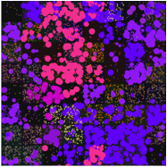
Figure 1. An illustration of the grid of 2D patches, in this case an 8x8 grid. Plants are small stars, herbivores and higher predators are circles (the more they have eaten the bigger they are up to a maximum size,). Different colours indicate different species but not all species are visually distinguishable.
Key to this simulation is understanding how it is determined whether individuals can extract energy from a patch or predate upon another. This method is adapted from that in (Caldarelli et al. 1998). A random interaction matrix with the dimensions of the length of individuals’ bit-strings is generated at the start of a simulation. It is filled with normally distributed random floating-point numbers (mean 0, standard deviation 1/3)[3]. This interaction matrix determines which entity can eat another entity in the following manner (see Figure 2 for an illustration):
1. The non-zero bits of the predator select the columns of the matrix, the non-zero bits of the potential prey select the rows.
2. The intersection of the selected rows and columns determine a set of numbers, these are summed.
3. If the sum is greater than zero the predator can eat the prey, in which case the prey dies and the predator gains a percentage of its energy value the rest is lost, .
Essentially the same process is used to determine which entities can extract energy directly from the environment, except that the part of the prey is taken by the patch with its bit string (padded with zeros to reach the appropriate length). In this case only those with scores greater than zero get any of the patch’s energy. The patch’s energy is divided between all qualifying individuals in proportion to their score against the patch. This scheme has the consequence that no individuals can extract energy from a patch with a bit-string of all zeros. Thus all the simulations reported below will have some patches that act as “deserts”, that is patches where individuals cannot extract any energy from the environment (although they may pass through the patch using previously stored energy or predate upon other individuals there).
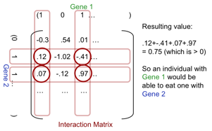
Figure 2. The use of the interaction matrix to determine predation as well as energy extraction from a patch to give its relative fitness.
This interaction scheme allows complex food webs to be evolved, for example via a genetic “arms-race” between predator species and prey species, since it allows for adaption with respect to another specific species. In other words fitness is not an absolute number but relative to the environment, if it extracts energy from this, or another species. (Caldarelli et al. 1998) showed that this kind of scheme can be used to evolve complex ecologies with plausible characteristics including food-webs with similar network characteristics to observed food-webs.
At the start of the simulation, the random interaction matrix is generated. Each patch is allocated a random bit-string with the given number of bits, padded out with zeros to make it the same length as individuals’ bit-strings, . The “environmental complexity” is the number of significant characteristics that patches have – the number of bits in its bit-string. Bit strings of length 2 allow for 4 types of patch, of length 3 8 types etc.[4]. The simulation starts with no individuals.
Each tick:
1. Input energy. A fixed amount of energy is added to the model, equally divided between all the patches.
2. Death. A life tax is subtracted from all individuals, if their total energy is less than zero it is removed from the simulation. Their age is incremented
3. Initial seeding. (In the initial phase), until a viable population[5] is established, a random new individual is introduced with a given probability.
4. Energy extraction from patch. The energy stored in a patch is divided among the individuals on that patch that have a positive score when its bit-string is evaluated, using the interaction as described above (against the patch’s bit-string) in proportion to its relative fitness, at the simulation’s efficiency rate, .
5. Predation. In a random sequence, each individual is randomly paired with a number of others on the patch, given by the parameter “eating tries”, . If it has a positive dominance score against the other, the other is removed from the simulation and the individual gains a fixed proportion of its energy, given by the “efficiency” parameter, . Individuals are not allowed to predate upon members of their own species.
6. Maximum Store. Individuals can only retain so much energy, so any above the maximum level set is discarded.
7. Birth. If an individual has a level of energy above that determined by the “reproduce-level” parameter, it gives birth to a new entity with the same bit-string as itself, with a probability of mutation, . The new entity has an energy level of 1, which is subtracted from the energy of the parent.
8. Migration. With a probability determined by the “migration” parameter, the individual is moved to one of the neighbouring 4 patches (the world being “wrapped” top and bottom).
9. Statistics. Various statistics concerning the model are calculated.
The simulation ends after a given number of ticks. At the end, the diversity of the ecology is calculated, this is the average hamming distance between all bit strings in the ecology[6], called “pi-t”, following (de Aguiar et al. 2009). This is a better measure of diversity than the number of species since it is not disproportionately influenced by the existence of almost extinct species.
Notable features of this set-up are:
· It can produce ecologies with plausible food webs.
· The fundamental interactions in the model, those that constitute the food chain, are emergent and can continually change in both time and space.
· The model creates endogenous shocks on its own, with new species appearing to sometimes-catastrophic effect on the existing food chains, affecting them radically in terms of their constituent species, their relative abundances and even the predation links.
· Mutation and migration happen in parallel, so that new species often appear before previous species have been completely spread over the space – states that could be interpreted as being in “equilibrium” are rarely observed, unless the ecology is non-viable or is dominated by a single species, .
2.2 Typical Behaviour of the Basic Simulation
There are four different ecological kinds of outcome observed in this model:, 1, a non-viable outcome where nothing thrives or reproduces, defined as being fewer than 10 individuals in the whole space, , 2, a situation where one, or two, plant species dominate, 3, a plant ecology, not case 1 or 2, with no herbivores or higher predators and, 4, a mixed ecology like case 3 but with herbivores and higher predators. In practice if there are fewer than 10 individuals there are usually one or no individuals within a few simulation ticks, and if there are either one or two species or many. Thus although the division is somewhat arbitrary, it very clearly distinguishes four cases between observed simulation trajectories. Furthermore these four kinds tend to persist for many simulation ticks so that each can be meaningfully identified. These are each described with outcomes from a typical run below. Many of the later results will be in terms of the occurrences of each of these four types.
Each description is accompanied with three figures (left) is a visualisation of the patches and individuals, the colours of the background patches indicates its bit-string, plants are indicated by a small star, individuals higher up the food-chain are indicated by a circle whose size is related to how many other individuals they have eaten; (centre) is a graph of the number of species over time; and (right) is a graph showing the number of individuals of each trophic level on a shifted log scale.
2.2.1 Non-Viable Ecology
Here species do not manage to extract any energy from the environment, so any introduced species quickly starve with no reproduction. There is only ever one individual since when this one dies a new random one is introduced into the simulation.
|
|
|
|

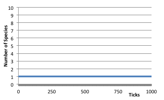
Figure 3. Typical Non-Viable Ecology (left) the world state (left) Number of Species (right) Log, 1 + Number of Individuals at each trophic level,
2.2.2 Dominant Species Ecology
Here one, or a few, species dominate. The dominant species is both a plant and a predator, eating any new other species that appear. Thus, occasionally individuals are classified as belonging to a higher order trophic level, although no other species manages to achieve a long-term survival. Very occasionally two or three dominant species occur, each destroying the others that wander into the patches they dominate.
|
|
|
|

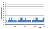
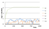
Figure 4. Typical Dominant Species Ecology (left) the world state (left) Number of Species (right) Log, 1 + Number of Individuals at each trophic level,
2.2.3 Rich Plant Ecology
In this case a rich plant ecology develops where many different species compete as to their efficiency in extracting energy from the different kinds of patch, and are resistant to potential herbivores who, if introduced, simply starve. In terms of the number of individuals this state often produces the greatest number of species and the highest population (in terms of number of individuals). Species only gradually replace older ones as they marginally out-compete them in terms of energy extraction.
|
|
|
|

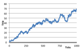
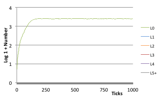
Figure 5. Typical Herbivore Ecology (left) the world state (left) Number of Species (right) Log, 1 + Number of Individuals at each trophic level,
2.2.4 Mixed Ecology
In the last case, successful herbivores and higher predators evolve to produce a highly dynamic ecology. There is a continual “arms race” both in terms of bit-string evolution as well as over the space of patches. There are typically far fewer species than in the rich plant ecologies since many plant species are wiped out. This typically results in a power law in numbers of individuals at each trophic level with an order of magnitude between the prevalence of each layer. Here you get a more constant replacement of older species as found in (Drossel et al 2001).
|
|
|
|

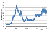
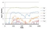
Figure 6. Typical Mixed Ecology. (left) the world state (left) Number of Species (right) Log, 1 + Number of Individuals at each trophic level,
2.2.5 Sensitivity Analysis of Basic Ecological Model
Each individual run of this simulation can give very different results starting from the same parameter values. Partly this depends on the interaction matrix generated and partly on the happenstance of mutation and movement within the world. Summaries of such runs for different parameter values may thus be misleading as averaging may give a false picture of the collection of trajectories. Thus for each parameter I show both the average effect on diversity over all the runs, the charts on the left below (with a 95% spread) but also a count of how many runs end up in each of the four states above (the bar-chart on the right below). For each of these there were 25 runs of 1000 time ticks for each parameter value. Where the results are less interesting I have relegated the graphs to Appendix II.
|
|
|
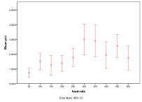
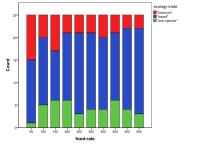
Figure 7. Effect of Energy Input on (left) diversity and (right) ecological type red=plant, blue=mixed, purple=single species, green=non-viable
The more energy that is put into the system then, generally, the greater the diversity that results (Figure 7), however the response to more energy is non-linear as larger populations support more predators, which has the effect of reducing the diversity. Generally, the higher the input energy, the less frequent does a pure plant ecology result.
|
|
|
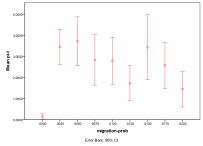
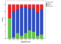
Figure 8. Effect of Migration Rate on (left) diversity and (right) ecological type red=plant, blue=mixed, purple=single species, green=non-viable
A zero rate of migration means that each patch is isolated, so this severely restricts the diversity and ensures small populations. Above that the higher the migration rate, the lower the diversity since patches act less like semi-isolate demes and more like a total well-mixed population, with all species competing against all (Figure 8).
|
|
|
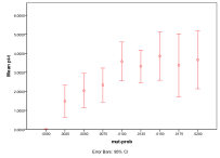
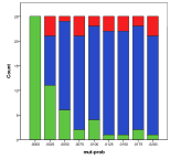
Figure 9. Effect of Mutation Rate on (left) diversity and (right) ecological type red=plant, blue=mixed, purple=single species, green=non-viable
A zero mutation rate means that nothing can evolve, so that there is, at most, one species. Above that, a higher mutation rate implies a higher diversity and fewer cases of a “single species” ecology (Figure 9).
|
|
|
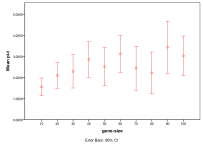
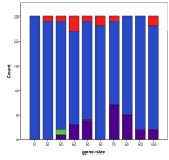
Figure 10. Effect of Gene Size on (left) diversity and (right) ecological type red=plant, blue=mixed, purple=single species, green=non-viable
Longer bit-strings enable a greater diversity to develop, however the space of possibilities is so great for sizes above 40 that this is nowhere near explored and hence does not limit the growth of complexity at these scales of space and time, Figure 10, .
|
|
|
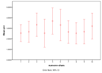
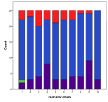
Figure 11. Effect of Environmental Diversity on (left) diversity and (right) ecological type red=plant, blue=mixed, purple=single species, green=non-viable
Greater environmental diversity seems to decrease the occurrence of rich plant ecologies, Figure 11, .
|
|
|
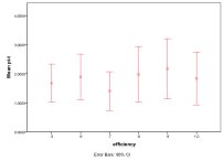
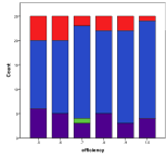
Figure 12. Effect of Efficiency on (left) diversity and (right) ecological type red=plant, blue=mixed, purple=single species, green=non-viable
Higher efficiencies mean that ecologies with higher trophic levels occur more often, since the higher levels can access more energy, Figure 12, .
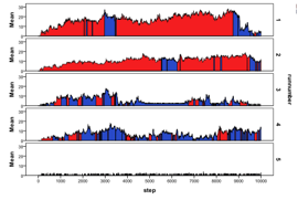
Figure 13. An illustration of the number of species and the types over longer runs, red=plant, blue=mixed
During longer runs, the simulation is often observed to change state between the types of ecology listed above.
Figure 13 shows 5 independent runs of the model over 10,000 simulation ticks with a lower mutation rate, 0.001, . The first two runs are dominated by plant ecologies with occasional periods of higher tropic levels appearing, the second two are the reverse and remain mixed ecologies for the majority of the time, though mixed ecologies are not as stable as plant ecologies, . The last is dominated by a single species and remains so with very short-lived appearance of herbivores. These longer runs illustrate the long-term robustness of the four types of ecology in this model. In the top two runs illustrated in Figure 13 a rich plant ecology dominates, sustaining large numbers of individuals, with occasional short-lived intrusions of herbivores. In the next two runs a mixed ecology dominates with occasional periods when herbivores disappear. The bottom run shows the stability of the situation when one species dominates, effectively preventing any others appearing.
2.3 Discussion
To summarise, the basic model provides a complex and dynamic representation of an ecology of species that has an ability to evolving in response to changes across a somewhat complex 2D landscape of different types. This makes it an ideal base in which to investigate some of the possible complex ways in which ecologies could be affected by systemic change.
3. Adding in the impact of humans via interference in the underlying species interaction
The first approach to modelling the systemic impact of humans is by altering how the interaction matrix is applied. The idea behind this is that, due to the interference of humans in the environment, some of the ways in which species interacted might be no longer available to them – this aspect is “blocked”. Here the impact of humans is via how this changes how species can interact. This is intended as an exploration a relatively short-term impacts.
3.1 The Method
The starting point for the experiments here is a mixed ecology that appeared 2200 ticks into a simulation. Its “trajectory” up to this point is shown in Figure 14, and the distribution of the trophic levels in Figure 15.
It is from this state that, repeatedly, the effect of blocking different interaction aspects and using different random seeds, from this point on, . Thus the following happens:
· For each aspect to be blocked, none, 1,… aspect 16, :
o Repeat 100 times:
§ The simulation is “rewound” to this point
§ Measure the diversity of the whole world and each kind of patch
§ Run forward 100 more steps using a different random seed
§ Re-Measure the diversity
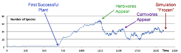
Figure 14. The evolution of the mixed ecology used as the starting point for exploring the impact of changes in the interaction structure of species
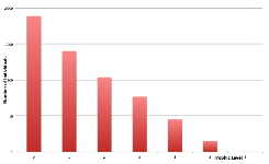
Figure 15. Trophic Levels at Frozen Starting Ecology
The “blocking” mechanism works as follows. Suppose aspect 3 was to be blocked, then every time the interaction matrix is used to calculate whether one individual can predate on another, or whether an individual can extract energy from a certain patch, , then the bits at position 3 in both bit-strings would be temporarily forced to zero. Thus the calculation would be done as if all bits at position 3 were 0 and hence the numbers in column 3 or row 3 of the interaction matrix would not form part of the sum that determines whether energy can be extracted from another, individual or patch, . Thus blocking simply removes this dimension from any significant part of the simulation, globally changing the structure of interaction from this point onwards. It is the differences in the diversity measures after 100 time clicks that we are interested in, since here we are only interested in the short-term impact and not that over evolutionary time.
3.2 Results
Figure 16 summarises the changes in diversity over this time. The first bar in Figure 16 is a summary of the null case – when no aspect was blocked. Unsurprisingly sometimes the genetic diversity drifts up and sometimes down, with the average change being very close zero. The next 16 bars summarise the effect of blocking each aspect in turn. On can see that, although in many cases it does not seem to make a significant difference, for some aspects it causes a significant increase in diversity (aspects 1 and 2) and others a significant decrease (aspects 9, 10 and 16). If one averages over all blocking runs, regardless of which aspect is blocked, one gets the results summarised in the far right bar, which is almost indistinguishable from the null case. If one had only looked at this summary one might have, wrongly, concluded that there was no risk from interfering with the interaction structure of species. However, it does seem to be unpredictable what the effect will be for each aspect.
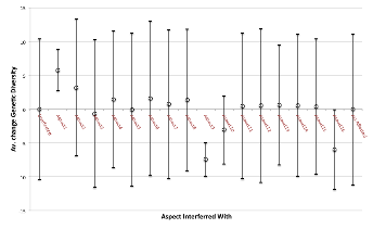
Figure 16. Summary of Impact of “blocking” different aspects of interaction after 100 more simulation ticks, (results summarise 100 runs for each aspect)
The next two figures show the same results by each type of patch. Figure 17 is displayed by aspect sorted into the average impact blocking over all types. One can see that for a range of aspects, those in the middle of Figure 17, there is almost no effect of blocking it, in that the impact is indistinguishable from the no blocking case. In these cases the aspects blocked has no overall impact upon the interaction of species. There are three aspects which if blocked have a generally negative effect upon diversity across most patch types and four which have a generally positive effect upon diversity if blocked. Figure 18 shows the same data but arranged by patch type with a different symbol for each aspect blocked. It is notable that the impact of blocking differs considerably between patch types, there are some patch types where the impact is generally positive whichever aspect is blocked and some where the impact is generally negative.
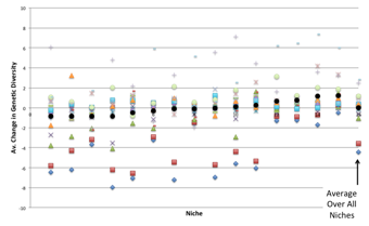
Figure 17. Average change in diversity by patch type sorted in order of average impact across all aspects blocked (each symbol representing the change due to changing a different aspect)
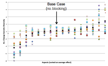
Figure 18. The change in diversity due to blocking on each type of patch sorted by aspect in order of the average impact (each type of patch is represented by a different symbol)
3.3 Discussion
This exploration of the impact of changing the underlying structure of species interaction in the short term generated no global trends. Rather, the impact of blocking one dimension of interaction had very different impacts upon different patch types and different patch types were impacted in different ways by blocking different aspects. An overall summary of the impact would mask this doubly differential impact, since even if the overall average impact was neutral particular patches could be greatly perturbed by when specific aspects were blocked, adding local environmental shocks into the system. This shows the possibility that even if systemic change does no have an obvious impact in terms of global statistics this might mask quite dramatic effects within certain niches, in both positive and negative directions. Such perturbations, when combined with other shocks, might be catastrophic for local niches, wiping some out and completely changing others.
4. Exploring the impact of humans via introducing agents representing them into the basic model
The second method of simulating the impact of humans upon the basic ecology is by injecting them as agents into the model once a basic ecology has had a chance to establish itself. This method embeds the impact of humans within the model, rather than as an exterior intervention. It allows the dynamics of the participant individuals of an ecology to be explored as a whole system, thus enabling the identification of dynamics that might not be manifest from examining that of the ecological system or human system alone, or by connecting models of an ecology and human system via simple connection (e.g. only the numbers of each impacting on the other).
4.1 Method
The agents representing humans share many aspects of the entities in the basic ecological model.
· They have a similar bit-string of characteristics representing their abilities and these are assessed against other species in the same manner as before using the interaction matrix.
· They inhabit the grid of patches and can migrate to neighbouring patches as other entities.
· They have a similar energy economy as other entities.
· To survive they have to successfully predate upon other entities. They may be predated upon by other entities.
However, there are important differences.
· They are not allowed to extract energy directly from a patch, even if their bit-string would allow this, but have to eat plants and other entities around to survive.
· Their bit-string is not genetic, but rather represents a set of skills that can be changed during a lifetime. Change in the bit-string does not particularly occur at birth since these skills are passed to children during training, but rather there is a relatively high rate of continual change in their characteristics throughout the life of human individuals.
· They can learn from nearby other humans on the same patch as themselves. That is there is a probability that they look at a set number of other random humans on the same patch, and if they have more energy than themselves, they copy a random bit from them.
· The rate of change of their bit-strings is higher than that of other entities, since it represents a cognitive rather than genetic process.
· They arrive in the simulation as a diverse group of individuals on the same patch, if these die out another group is introduced after a period of time, .
· Some of their parameters are also different: they have a max age of 100, a higher threshold for reproduction, 20, , and a higher default ability to store energy, 30, .
· In some of the runs reported below their migration rate is different than for other entities allowing the exploration of the effect of the relative rate of migration rates.
These agents are not just another predator; they are not restricted to a genetic mutation rate at the same rate of their prey but can adapt far more quickly and then share these adaptions with their peers. In this way they change the pattern of evolutionary competition and, if they survive, can easily dominate the ecosystem. These agents might be interpreted as representing hunter-gatherer nomads who indiscriminately eat what happens to be around and then move on to a new location.
4.2 Results
Here we deliberately give results from a number of different levels and methods.
4.2.1 Some Typical Trajectories
There seem to be a variety of different kinds of trajectory possible once human individuals have been introduced into the model.
One possibility is that humans do not manage to predate upon any existing organisms and rapidly die out. In this case they have little impact upon the ecology. Another is that they predate only upon a thin top layer of herbivores/predators and then die out after they have eliminated any of those around themselves. This has the effect of a temporary depression in the numbers of these, which recover as soon as the human individuals have gone. These are not illustrated since they are obvious.
A third, more catastrophic possibility is that the humans predate upon all the entities in the simulation, allowing a population explosion that eventually results in the consumption of all other entities in the world, after which the human agents gradually starve. This is the sequence illustrated in Figure 19.
|
|
|
|
|
|
|
|
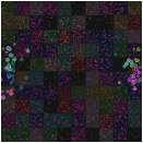
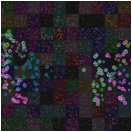
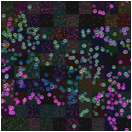
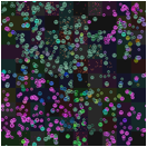
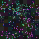
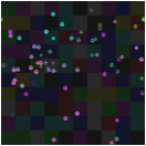
Figure 19. A sequence of world snapshots of an invasion of humans into a plant ecology with fast migration, causing self extinction due to elimination of plants
A fourth possibility is that some kind of spatial predator-prey dynamics emerge for a while between humans and other entities. An illustration of this is in Figure 20. Here “waves” of humans develop, consuming all in their path but in such a pattern that new clumps of entities develop in the patches they have disappeared from (due to the previous elimination of food). This is a spatial “cat and mouse” situation, which depends upon the humans not spreading evenly but accidently leaving patches and those patches being able to be seeded by other entities and thriving for a short time there.
|
|
|
|
|
|
|
|
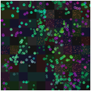
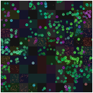
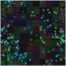
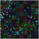
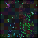
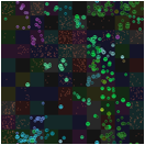
Figure 20. A sequence of world snapshots with slower migration with humans eating all resources as they go, but new plants re-growing after they have left
A graph of their numbers may look like classic predator-prey dynamics such as in Figure 21, although this apparently simple summary might not reflect what is happening within a more complex spatial dynamic.
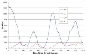
Figure 21. Number of humans and plants in a single run of the simulation starting from a rich plant ecology, from the point at which humans were introduced.
There are, of course, more complex mixes of dynamics where the pattern is not so distinguishable to the eye.
4.2.2 Sensitivity of model with and without humans
The first set of results is a series of runs where the ecology is allowed to evolve without humans for 1000 ticks, as described above, and then in half the runs people are injected as a diverse group of 50 people into one patch. If the people die out then after 100 ticks, giving the ecology a chance to recover, another batch of people is injected. If there are any existing people then no new people are injected from the outside. The simulation continues to time 2000, when the statistics are calculated: the kind of ecology that it is at this point and the measure of diversity. This is done 25 times for each parameter value with humans and 25 without.
|
|
|
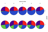
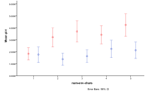
Figure 22. The differential effect of the
arrival of humans, or
not, (left) by proportion of ecology types, red=plant, blue=mixed, purple=single species, green=non-viable (right) by diversity of ecology, blue=with humans, red=without
In Figure 22 we look at the effect of the presence of humans in environments of different complexities, measured by number of different patch types, . Humans have a general depressing effect upon the ecological diversity. Without humans, increasing environmental complexity means fewer cases of herbivore ecologies, but with humans the incidence of herbivore ecologies increases with environmental complexity. Whilst environmental complexity increases the proportion of mixed ecologies without people but is roughly constant with people.
|
|
|
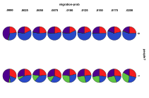
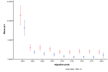
Figure 23. The differential effect of the arrival of humans, or not, with, entity and human, migration rate (left) by proportion of ecology types, red=plant, blue=mixed, purple=single species, green=non-viable (right) by diversity of ecology, blue=with humans, red=without
In Figure 23 we look at the effect of different migration rates (the same for entities and humans). As before a zero migration rate is catastrophic because entities and humans never spread beyond a single patch. Without humans the migration rate does not have much effect on the occurrence of ecology types, but with humans increasing migration rate results in more non-viable ecologies at the expense of mixed ecologies.
|
|
|
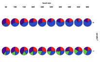
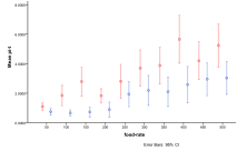
Figure 24. The differential effect of the
arrival of humans, or not, with availability of energy (left) by proportion of
ecology types, red=plant, blue=mixed, purple=single species, green=non-viable (right)
by diversity of ecology, blue=with humans, red=without
Figure 24 shows the differential effect of the amount of energy being input into the system. Without humans an increase in energy allows for more diversity and a greater occurrence of mixed ecologies and fewer plant and single species ecologies. With humans increasing energy results in more mixed ecologies but also many more non-viable states, due to the human population growing faster than the ecology and wiping out their own food supply.
4.2.3 A Larger Random Sample of Runs with Humans
4,478 runs of the simulation, starting from a blank ecology at tick zero with humans entering at tick 1000, running the simulation on to tick 2000 were performed with parameters set at random from given ranges, world dimensions from {2x2, 3x3,… 10x10}; number of patch types from {2, 4, 8, …, 32}; migration rate from {0, 0.0025, 0.005,…, 0.02}; energy input rate from {50, 100, …, 500}; innovation rate from {0, 0.05, 0.1,…,0.2} and learning rate from {0, 0.1}, . The purpose of this is to enable the exploration of factors not in a ‘thin’ slice of parameter sampling but over a wide variety of settings, as would be the case in observed ecologies, . Thus these results are less like a controlled experiment and more like observing a large number of occurring cases to look for trends, as might happen to field data. Thus the results in this subsubsection correspond to data-mining observed data which might display more of the natural variety that such data would contain (covering a wider range of cases).
|
|
|
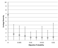
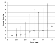
Figure 25. Overall change in ecological diversity with humans being introduced with (left) migration rate and (right) energy input into the system.
Figure 25 shows the overall change in diversity across all final states analysed by migration rate and amount of energy available to the system. Increasing migration rate has the effect of decreasing diversity due to more mixing but also faster spread of humans to patches with other entities on them. A greater amount of energy input does result in a higher level of average diversity but with a greater spread of outcomes as energy increases.
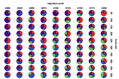
Figure 26. Proportion of different ecological
outcomes with humans for different migration probabilities and food rates, red=plant, blue=mixed, purple=single species, green=non-viable
Figure 26 splits the results according to rate of migration and the input energy, with the proportion of each kind of outcome displayed. There is a greater proportion of single species outcomes for low rates of energy input and input energy. For low mutation rates increasing the energy available increases the proportion of mixed ecologies, but for high mutation rates more energy increases the proportion of non-viable outcomes.
|
|
|
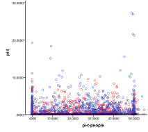
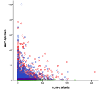
Figure 27. Diversity (left) and number of
species/variants (right) of people,, horizontal axes, and other entities, vertical axes, , red=plant, blue=mixed, purple=single species, green=non-viable
Figure 27 is a scatter plot of all outcomes in terms of ecology diversity and then number of variants/species. In terms of diversity there are all levels of diversity in the human bit-strings whilst the ecological diversity is limited to smaller levels, the presence of people severely depresses ecological diversity (up to a maximum carrying capacity for people). When the number of variants among human agents is plotted against number of species we see that one rarely gets a high number of variants at the same time as a high number of species – species and variants seem to be mutually exclusive.
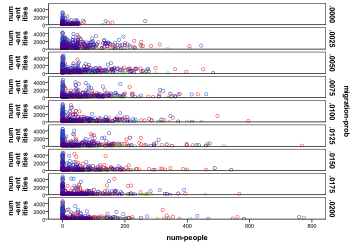
Figure 28. Number of species/variants of
people by different migration probabilities,, horizontal axes, and other entities, vertical axes, , red=plant, blue=mixed, purple=single species, green=non-viable
Figure 28 is a scatter graph of the sheer numbers of people and entities by different migration rates. At low, but non-zero, migration rates we see cases with relatively high numbers of entities and people but for high migration rates there are fewer of these cases, with a tendency to result in very few people or very few entities.
4.2.4 Starting from a given Ecological State
Here, three contrasting ecological states were “saved”: a rich plant ecology, a single species plant ecology, and a mixed ecology with all trophic levels. Then two sets of simulation runs were one where migration rates for entities and humans were varied systematically and one where innovation rates for humans and mutation rates for entities were varied. 25 simulations starting at the same ecological state where done for each parameter up to 2000 ticks, ecology was “frozen” at 1000 ticks, and the type of ecology stored. These results are now discussed.
|
|
|
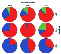
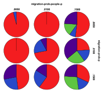
Figure 29. Starting from a Plant Ecology the effects
of innovation rate/mutation rate (left) and people migration rate/entity
migration rate (right) , red=plant, blue=mixed, purple=single species, green=non-viable
Figure 29 shows the outcomes starting from the same plant ecology. Unsurprisingly plant ecologies still tended to dominate after 1000 ticks. Higher mutation rates and lower innovation rates resulted in more mixed ecologies resulting. When the migration rate of people was less than or equal to that of other entities more mixed and single species ecologies resulted. A higher proportion of non-viable states occurred with low levels of entity mutation and high levels of human migration.
|
|
|
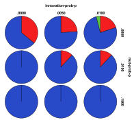
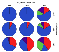
Figure 30. Starting from a Mixed Ecology the
effects of innovation rate/mutation rate (left) and people migration
rate/entity migration rate (right) , red=plant, blue=mixed, purple=single species, green=non-viable
Figure 30 shows the outcomes starting from the same mixed ecology. Again mixed ecologies still tended to dominate after the arrival of people. Low levels of entity mutation or high levels of entity migration resulted in a greater proportion of plant ecologies. Again high rates of people migration resulted in a greater proportion of non-viable states, but this time a low level of entity mutation did not result in many non-viable states.
|
|
|
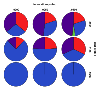
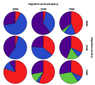
Figure 31. Starting from a Single Species
Ecology the effects of innovation rate/mutation rate (left) and people
migration rate/entity migration rate (right) , red=plant, blue=mixed, purple=single species, green=non-viable
Figure 31 shows the outcomes starting from the same single plant species ecology. Here a high level of entity mutation resulted in the appearance of mixed ecologies and high levels of either entity or people migration resulted in the appearance of more plant ecologies. High levels of both entity and people migration rates resulted in a higher proportion of non-viable states.
Consistently, regardless of the starting ecological state, a high rate of people migration resulted in a greater proportion of non-viable states and higher mutation rates results in more mixed states. However the effects of varying these parameters were also different depending upon the ecological state started from. Both rich plant and mixed states were more resistant to being altered into a different state, in other words more resilient to the impact upon humans (in terms of type).
4.3 Discussion of Results
In this model, the human individuals had a profound, but sometimes complex, effect upon the ecologies they entered.
In terms of straightforward effects there was the following. They uniformly reduced ecological diversity, causing a greater proportion of non-viable states and far fewer mixed ecologies since they directly competed with herbivores and higher predators. They often caused their own disappearance as they wiped out the species they depended upon for sustenance. High levels of migration reduce diversity (Figure 23, Figure 26, Figure 28, Figure 29, Figure 30 and Figure 31). The greater the migration rate between patches the less they act as separate demes, which afford some protection of the diversity.
In terms of more subtle and context-dependent effects there were the following. The presence of human individuals flattened the effect of increasing environmental complexity. So whereas increasing the number of patch types would result in an increase in environmental complexity, in the presence of humans this effect is almost eliminated (Figure 22). The presence of humans also changes the impact of increasing energy into the environment, from increasing mixed states, decreasing single species and plant states, to increasing non-viable states, decreasing single species states, (Figure 23). Species diversity is somewhat of a short-term protection against the arrival of humans since each group of humans might not be able to predate upon all kinds of species simultaneously, leaving certain species less affected until a different group of humans sweeps over the world. Higher mutation rates among non-human entities ensure a higher supply of new species to the world and hence tend to result in more diversity (Figure 24), a greater proportion of mixed ecologies and no non-viable ecologies (Figure 29, Figure 30 and Figure 31). Since each mixed patch is usually dominated by humans or other entities and not both for extended periods of times (Figure 28).
In terms of starting from each of three different kinds of ecology with humans being injected we had the following results.
Richer plant ecologies (Figure 29) tended to remain so for medium/low mutation rates, and lower migration rates (both entity and human). For high mutation rates they often evolved into mixed ecologies even in the presence of humans. High migration rates meant that it could evolve into any of the states. Low mutation rates or high people migration rates also meant a proportion became non-viable.
Mixed ecologies (Figure 30) were also fairly stable, tending to remain almost entirely for high migration rates for both humans and entities. Low mutation rates or high entity migration rates increased the tendency to result in a herbivore state.
Single species states (Figure 31) were the most vulnerable to change and less so the higher the mutation rate and migration rates. For high mutation rates they had a strong tendency to result in a mixed ecology, for medium/high migration rates they tended to result in a herbivore or non-viable state.
These indicate that transition probabilities between ecological states would be highly dependent upon factors such as mutation and migrations rates. Mixed ecologies seem to be facilitated by high mutation probabilities, allowing ecologies to adapt to changing humans better (sometimes avoiding their predation), low migration rates of people and others, in situations of low mutation rates a lower innovation rate helped. Non-viable states most often arose from high people migration rates, and low mutation rates when starting from a plant ecology.
5. General Discussion
In any complex system where change is endogenously embedded, it will be hard to identify “the” cause of any particular outcome. As pointed out before (Edmonds 1999) such simulations, and presumably many systems that we observe, are subject to the phenomena of “causal spread” (Wheeler and Clark 1999) whereby the further you trace the formal causes of any outcome back in simulation time via the firing of individual simulation rules, the set of causes can spread to include almost all entities and settings of the simulation. This is particularly hard when systemic change is endogenised, rather than applied from the outside as a parameter change or extra process.
One response to such complexity is to seek to simplify the model so that it can be rigourously understood. Clearly there is a tension between a wish for rigour (which almost always implies simplicity) and relevance (which almost always implies complication). This issue has been discussed elsewhere (Edmonds and Moss 2005). However in the case of wishing to explore some of the ways in which a system can fail, especially when one wishes to explore complex routes to failure (where it will be infeasible to track the complex web of interactions mentally), then one should err on the side of complication, since it often better to suffer a few false alarms, where one has identified a trajectory that, in fact, was harmless, rather than miss a possible danger. This explains the approach taken in this paper, since I am not concerned with predicting the probable but rather to capture and understand the possible.
In particular it no good hoping for clean universal laws from complex evolutionary systems. In this case both ecological systems and social systems are well known for displaying highly context-dependent patterns of behaviour (Edmonds 2012a). Accepting this does not mean that one has abandoned solid science, but rather have accepted the complexity (Edmonds 2012b). A far more insidious, and I would argue less productive, strategy is to limit oneself to using simple computation models that give an illusion of generality because they can be analogically applied to many situations. Analogies are very valuable for suggesting new insights but they are not falsifiable. Complex, specific and contingent but formal models with definite referents are amenable to inspection, critique and confronting with evidence. Thus they hold out the possibility of participating in the development of observation and understanding, slowly bootstrapping understanding over time (Edmonds 2010). I hope that the approaches and models described herein can be part of such a process.
Here it has been necessary to impose some level of interpretation upon the results to help understand the outcomes and be able to draw some conclusions from it (in the form of characterising and then counting kinds of outcome)[7]. Here it was necessary to go beyond simple relationships of changing parameters and measuring outcomes, since these necessarily were averages over a wide range of actual trajectories (even when limited to a single set of parameter settings). Rather some of the more telling outcomes were gained by being less general and looking at more specific outcomes, for example by starting the simulation at a particular “frozen” state and looking at a particular projection of a larger space of possible outcomes (as in Figure 29, Figure 30 and Figure 31). In this case the interpretations were drawn from observations of the simulations as a whole and not linked to the kind of systemic change engineered into them.
One direction that this work implies is the increased use of careful data-mining techniques in order to do more systematic explorations of the complex space of outcomes that such models output. This is an example of the strategy of “staging” the abstraction process from complex systems and maybe allowing a clustering and division of the analysis into different phases as appropriate (Edmonds 2012b).
Clearly there is a lot of possible further exploration and development of these kinds of model. Indeed the paper has only had room to describe some of the facilities and features of the actual simulation code[8]. Future possible developments include: exploring much larger simulations in terms of number of individuals, patches and time horizons; adapting the settings and arrangement of the simulation to be more representative of a particular ecology; an exploration of more sophisticated kinds of humans such as those that emerge separate groups using tag-like mechanisms (Holland 1993, Hales 2000); simulating more static farmers and hunters that have a fixed base but range further afield for prey.
6. Conclusions
An individual-based meta-population model of an ecology has been exhibited that has allowed for the exploration of some possible complex impacts of humans. This impact was approached in two different ways, once suitable for short-term impact analysis and one more suited to longer-time frames. These showed how the limiting oneself to a simpler model and keeping to high-level generic results might miss the possible specific impacts to particular niches and under particular circumstances. In other words, it showed how context-dependent the impact can be.
It instantiated in a computer simulation the following phenomena (and thus made them amenable to exploration):
· that humans generally can significantly reduce ecological diversity, with a particular impact upon higher trophic levels;
· that such nomadic patterns of resource usage by humans can destroy the ecology they depend upon;
· that higher levels of migration can help destabilise ecologies and help reduce diversity;
· that the presence of humans may nullify the advantages of environmental diversity, becoming themselves the key environmental factor.
It also suggested the following hypotheses concerning how people might impact upon such ecologies, namely that the presence of humans may:
· have a varied impact upon different niches, perturbing some of these significantly (increasing as well as decreasing diversity in different cases);
· modify the effect of different levels of available energy facilitating the development of non-viable ecologies even in high energy situations;
· that the kind of ecological state one is in changes the outcomes one might expect from it under different circumstances (e.g. migration rates)e;
· that catastrophic non-viable ecological states might be more likely in the presence of these kinds of human agents when there is a high degree of movement of people and entities and fewer sources of environmental diversity.
Finally, the very different transition probabilities and wirings between states in different settings casts doubt on the efficacy of simple state-based or system dynamics models to capture the possible routes to ecosystem failure.
7. Appendix I – More Details of the Simulation
A complete ODD description of the simulation is underway and will be posted with the model on openabm.org when finished.
7.1 Simulation Lineage
The simulation here can be seen as an ancestor of (Norling et al. 2008). It uses a variety of the interaction matrix described in (Caldarelli et al 1998). It relates to the ecological model described in (Edmonds 2013) but has only one type of basic resource.
7.2 Dominance Calculation
If the potential predator bit-string is represented by
vector ![]() ,
the potential prey (or patch) bit-string is represented by vector
,
the potential prey (or patch) bit-string is represented by vector ![]() and the interaction matrix by
and the interaction matrix by ![]() with entries
with entries ![]() then
then
![]() is calculated. In the case of a potential predator-prey
interaction predation (between individuals that are randomly paired within a
patch) occurs if
is calculated. In the case of a potential predator-prey
interaction predation (between individuals that are randomly paired within a
patch) occurs if ![]() and in the case of individual patch will
receive a share in the energy of the patch in proportion to s if
and in the case of individual patch will
receive a share in the energy of the patch in proportion to s if ![]()
7.3 Parameters
7.3.1 In the Basic Ecological Model
The parameters of the basic ecological model are as follows, with their default values in square brackets. Note that not all of these are explored in the paper, but simply left at their default values.
· gene-size: [100] the number of bits in an individual’s gene
· num-env-chars: [3] the number of, effective, bits in the characteristics of a patch, functions similar to an individual’s gene,
· migration-prob: [0.01] the probability that any individual will move to another patch each time click
· mut-prob: [0.01] the probability that a newly born individual will have its gene mutated
· food-rate: [500] how much energy is put into the world each time click, evenly divided among patches,
· efficiency: [0.9] what proportion of energy of something eaten goes to predator, or to herbivore from patch,
· reproduce-level: [3] if an individual’s energy gets to this point it gives birth once, new-born’s energy being then subtracted from it,
· eating-tries: [2] each tick each individual tries to eat this number of others on the same patch, but this only happens if they dominate them via the interaction matrix
· max-age: [80] if > 0 individuals die when they reach this age in simulation ticks, otherwise no age ceiling,
· max-store: [20] if > 0 this is the upper bound on what energy individuals can accumulate, rest is lost to system,
· max-time: [1000] if > 0 the time at which the simulation is halted
The following are included for completeness but are not varied in the simulation runs reported.
· life-tax: [0.25] how much energy subtracted from each individual each time click, dies if energy is 0 or below,
· init-energy: [1] the energy of a new born, this is subtracted from the parent at birth,
· init-new-species-prob: [0.01] probability of a new individual with a random geneome being introduced each time click
· stop-new-species-once-established?: [true] if set stops new individuals with new genomes being introduced into the simulation once a viable population is established
· initial-species-variety: [0] 0/1: if 0 simulation starts with a single individual, if this is not successful relies on a new individual being intyroduced via init-new-species-prob, , if 1 starts with a full population with random genes
· rand-death-prob: [0.02] the probability an individual randomly dies each tick
· anti-sym-mat?: [false] forces the interaction matrix generated at start to be anti-symmetric
· migrate-near?: [true] if true then individuals migrate, if they do, to a neighbouring patch if false to a random other patch
· allow-cannibals?: [false] if true individuals of the same species can eat each other, if not can only eat those of another species
· neutral?: [false] if true then all individuals on a patch get the same amount of energy from the patch regardless of their bit-string, otherwise they have to dominate the patch via the interaction matrix to extract energy,
7.3.2 In the Extended Mode with Human Agents
· init-variety: [1] whether humans enter as a diverse of set of individuals (1) or a homogeneous set (0)
· tol-on?: [false] whether the tag-based tolerance system is turned on (allowing the emergence of subgroups) or off (in which case learning and sharing can happen with any humans in the same patch, that is tags are ignored)
· max-age-people: [100] if > 0 human individuals die when they reach this age in simulation ticks, otherwise no age ceiling,
· max-people-store: [30] if > 0 this is the upper bound on what energy humans individuals can accumulate, rest is lost to system,
· reproduce-level-people: [30] if a human individual’s energy gets to this point it gives birth once, new-born’s energy being then subtracted from it,
· innovation-prob: [0.009] the probability a bit in a human individual’s bit-string is flipped each simulation tick for each human
· learn-prob: [0.1] the probability an individual looks to another (elidgible) individual in the same area and (if it has higher energy than itself) copies one bit from it
· share-tries: [2] the number of times a human individual attempts to share any excess energy it has
· share-efficiency: [0.8] the proportion of energy that is transmitted during sharing (the rest is lost)
· min-share-level: [25] only energy above this value is shared if sharing occurs
· tag-mut-sd: [0.005] the standard deviation of the normally-distributed noise added to the tag during tag mutation
· tol-mut-sd: [0.005] the standard deviation of the normally-distributed noise added to the tollerance during tag mutation
· time-between-invasions: [100] the time after the last humans have died out that another injection of humans occurs
· people-enter: [1001] the tick that humans are first input into the simulation
· num-people-enter: [50] the number of human individuals input into the simulation at a time
· people-f-env?: [false] whether people are allowed to extract energy directly from a patch
· coop-radius: [1] the number of neighbouring patches that sharing and learning can occur over – can be just the patch (1), the patch and 4 neighbours (5), or the patch and all 8 neighbours (9).
· migration-prob-people: [0.01] the probability that a human individual will migrate
7.4 Platform and Code
The simulation and its code will be available from http://cfpm.org/models/ems from the 18th June 2013. Once the code has been cleaned and ODD documentation for this is complete it will be posted to openabm.org under the title “A multi-patch meta-population of an ecology with humans”.
7.5 Model Variants
There are four variants of the model explored here.
1. The basic ecological model
2. The variety that allows the blocking of individual aspects and the saving and loading of complete ecological states
3. The variation that includes the introduction of human individuals
4. The variation with humans that allows the random selection of parameter values within given ranges for multiple simulation runs
8. Appendix II – Auxiliary Graphs
Some graphs here are included for completeness.
8.1 From Section 2.2.5
Extra graphs from 2.1.5
|
|
|
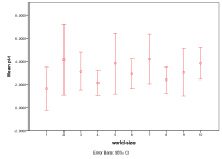
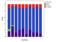
Figure 32. Effect of World Size on (left) diversity and (right) ecological type red=plant, blue=mixed, purple=single species, green=non-viable
Small world sizes, 1x1 and 2x2, result in more non-viable ecologies, and a lower diversity, Figure 32, . However, larger sizes have little effect on the basic model.
|
|
|
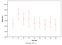
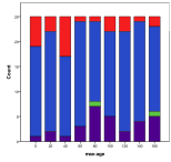
Figure 33. Effect of Maximum Age on (left) diversity and (right) ecological type red=plant, blue=mixed, purple=single species, green=non-viable, Note: Max. Age=0 means no maximum,
A maximum age setting of zero means no age limit in this model. Generally enforcing a lower maximum age helps diversity, since otherwise individuals that hoard large amounts of energy can exist for a long time, reproducing themselves, Figure 33, .
|
|
|
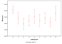
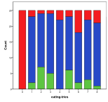
Figure 34. Effect of Number of Eating Attempts on (left) diversity and (right) ecological type red=plant, blue=mixed, purple=single species, green=non-viable
No eating attempts means that no energy can be passed up to a higher trophic level, but above that this has a mixed effect on diversity, Figure 34, .
8.2 From Section 4.2.2
|
|
|
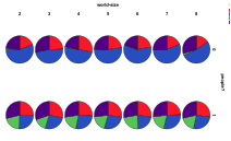
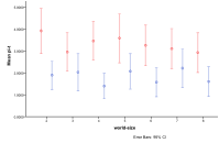
Figure 35. The differential effect of the
arrival of humans, or not, with world size (left) by proportion of ecology
types, red=plant, blue=mixed, purple=single species, green=non-viable (right)
by diversity of ecology, blue=with humans, red=without
|
|
|
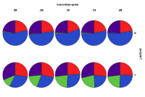
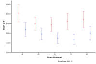
Figure 36.
The differential effect of the arrival of humans, or not, with human innovation
rate (left) by proportion of ecology types, red=plant, blue=mixed, purple=single species, green=non-viable
(right) by diversity of ecology, blue=with humans, red=without
|
|
|
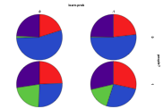
Figure 37. The differential effect of the
arrival of humans, or not, with learning rate (left) by proportion of ecology
types, red=plant, blue=mixed, purple=single species, green=non-viable (right)
by diversity of ecology, blue=with humans, red=without
8.3 From Section 4.2.3
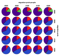
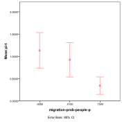
Figure 38. Proportion of different
ecological outcomes with humans for different migration probabilities for
entities, migration-prob,
and humans, migration-prob-people,
, red=plant, blue=mixed, purple=single species, green=non-viable
Acknowledgements
This research was partially supported by the Engineering and Physical Sciences Research Council, grant number EP/H02171X/1.
References
Caldarelli, G., Higgs, P.G. and
McKane, A., 1998. Modelling
Coevolution in Multispecies Communities. Journal
of Theoretical Biology, 193,
345-358.
de Aguiar, M.A.M., Baranger, M., Baptestini, E.M., Kaufman, L. and Bar-Yam, Y., 2009. Global patterns of speciation and diversity, Nature, 460, 384-387
Deffuant, Guillaume et al., 2012. Data and models for exploring sustainability of human well-being in global environmental change. European Physical Journal Special Topics, 214(1, , 519-545. DOI 10.1140/epjst/e2012-01704-2.
Diamond, J., 2004. Collapse: How Societies Choose to Fail or Succeed, Viking.
Drossel, B., Higgs, P.G., and Mckane, A.J., 2001. The Influence of Predator-Prey Population Dynamics on the Long-term Evolution of Food Web Structure. Journal of Theoretical Biology. 208, 91-107.
Edmonds, B. (1999). Capturing Social Embeddedness: a Constructivist Approach. Adaptive Behavior, 7:323-348.
Edmonds, B. and Moss, S., 2005. From KISS to KIDS – an ‘anti-simplistic’ modelling approach. In P. Davidsson et al., (Eds.), Multi Agent Based Simulation 2004. Springer, Lecture Notes in Artificial Intelligence, 3415:130–144.
Edmonds, B., 2010. Bootstrapping Knowledge About Social Phenomena Using Simulation Models. Journal of Artificial Societies and Social Simulation 13, 1, 8. http://jasss.soc.surrey.ac.uk/13/1/8.html,
Edmonds, B., 2012a. Context in Social Simulation: why it can't be wished away. Computational and Mathematical Organization Theory, 18, 1, :5-21.
Edmonds, B., 2012b (online first). Complexity and Context-dependency. Foundations of Science. DOI 10.1007/s10699-012-9303-x
Edmonds, B., 2012. Searching for “Phases” in Complex Simulation Output using Evolutionary Knowledge Discovery Techniques, (Poster) ECCS 2012, Brussels, Sept. 2012.
Edmonds, B. (2013) Multi-Patch Cooperative Specialists With Tags Can Resist Strong Cheaters. In Rekdalsbakken, W., Bye, R.T. and Zhang, H. (eds), Proceedings of the 27th European Conference on Modelling and Simulation (ECMS 2013), May 2013, Alesund, Norway. European Council for Modelling and Simulation, 900-906.
Hales, D., 2000. Cooperation without memory or space: Tags, groups and the prisoner's dilemma. In S. Moss & P. Davidsson, (Eds.), Multi-Agent-Based Simulation, 1979, 157-166.
Holland, J., 1993. The Effect of Labels, Tags, on Social Interactions. Working Paper 93-10-064. Santa Fe Institute. Sante Fe, New Mexico.
Norling, E., Powell, C and Edmonds, B., 2008. Cross-Disciplinary Views on Modelling Complex Systems. In. David, N. & Sichman, J.S., Eds., Multi-Agent-Based Simulation IX, Springer, Lecture Notes in Artificial Intelligence, 5269, 183-194.
Reader, J., 1990. Man on Earth. Penguin Books.
Terán, O., 2004. Understanding MABS and Social Simulation: Switching Between Languages in a Hierarchy of Levels. Journal of Artificial Societies and Social Simulation 7(4), 5. http://jasss.soc.surrey.ac.uk/7/4/5.html
Wheeler, M. and Clark, A., 1999. Genic representation: reconciling content and causal complexity. British Journal for the Philosophy of Science, 50 (1), 103-135.